
Component Reliability Analysis
Much of our work involves determining the reliability of components, where we want to understand how long they will last before failure. We use statistical analysis to predict these failures in terms of the expected number of hours used, miles driven, etc.
Say we are given data on vehicle components and how many miles were driven before the components needed to be replaced due to failure. We might want to know the average number of miles that a particular component was driven before it failed so that we would have a better idea of when a component of the same type would fail on a different vehicle. For example, this may help plan out regular maintenance on components with a shorter average lifespan, or help develop warranty periods of appropriate length.
Below is a graph of sample data on Component “A” failures:
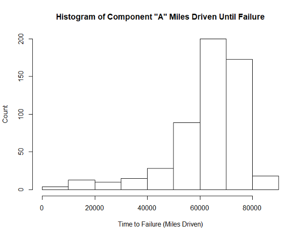
We can calculate the mean time between failures (MTBF) but note that it does not give us the whole picture, as the failures are not normally distributed. Luckily, we are able to fit this asymmetrical data using the Weibull distribution.
Weibull Distribution and Failure Rates Over Time
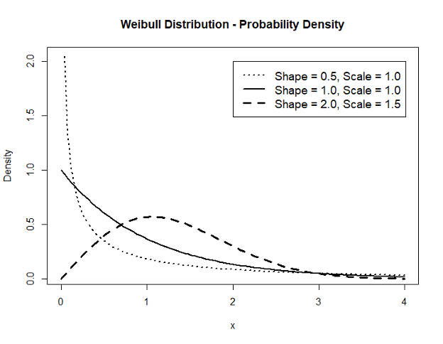
In reliability analysis, the most useful form is the two-parameter formula for the probability density function, where the time to failure is calculated using the two parameters shape and scale. This is a continuous distribution, theoretically with time going out to infinity. Time in this case represents miles driven. The shape parameter describes how the failure rate changes over time. If shape = 1, the failure rate is constant over time. If shape > 1, the failure rate increases over time, which is consistent with parts wearing out after longer usage. If shape < 1, the failure rate decreases over time, which is consistent with infant mortality of parts, where defective parts fail early before much usage and those that are left that did not fail early continue on to work as intended. The scale parameter simply adjusts the distribution to fit over the correct range of time, stretching the distribution wider or narrower.
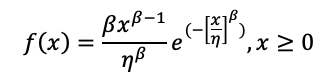
Below is the formula for the probability density function of the two-parameter Weibull distribution where shape is represented by β and scale is represented by η:
Changing the parameters changes the shape of the distribution:
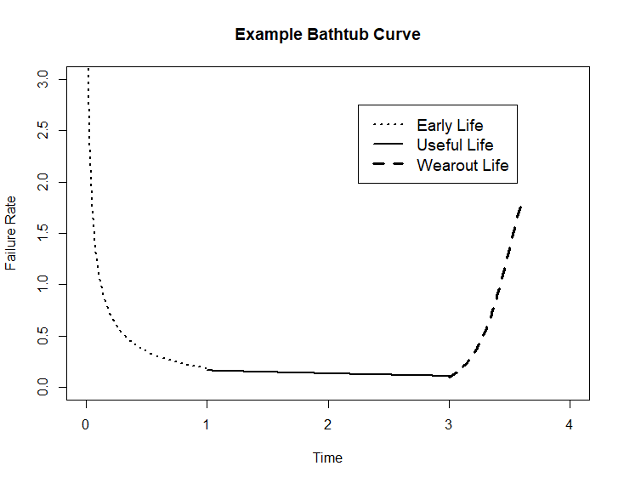
The classic “bathtub curve” to describe failure rate over time is a mix of three Weibull distributions fit the different subpopulations of parts. It is important to be aware that a single component can exhibit different patterns of failure rate over time, having both early-life failures and wear-out failures, and these would be described by two different Weibull distributions, three if we include a portion of constant failure rate time as well. Continually fitting subpopulations of components can also alert us to any changes in the reliability of components, for example observing if a new batch was exhibiting many early life failures.
Predictive Analytics to Enhance Decision Making
Perhaps we want to predict the probability of any vehicle component failing in the next 500 miles and it is currently in the shop for an oil change at 30,000 miles. If there are any parts that have a high probability of failing that soon then a potential solution would be to replace them while the vehicle is being serviced already, rather than wait until it fails. That is only part of the picture though, as each component has a real replacement cost and a cost associated with an unexpected failure. Overall, the fitted Weibull distributions can help make those decisions for many different users including manufacturers, fleet operators, and individual maintainers to balance out costs, improve safety, and manage maintenance resources efficiently.
Are you interested in understanding how statistical analysis drives real decisions? Contact us to learn more.